Search the handbook:

⇐ Previous topic|Next topic ⇒
Table of Contents

---

Analysis of covariance

---

Summary

Use analysis of covariance (ancova) when you want to compare two or more regression lines to each other; ancova will tell you whether the regression lines are different from each other in either slope or intercept.

When to use it

Use analysis of covariance (ancova) when you have two measurement variables and one nominal variable. The nominal variable divides the regressions into two or more sets.

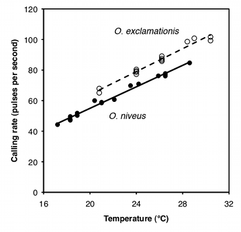
The purpose of ancova is to compare two or more linear regression lines. It is a way of comparing the Y variable among groups while statistically controlling for variation in Y caused by variation in the X variable. For example, Walker (1962) studied the mating songs of male tree crickets. Each wingstroke by a cricket produces a pulse of song, and females may use the number of pulses per second to identify males of the correct species. Walker (1962) wanted to know whether the chirps of the crickets Oecanthus exclamationis and Oecanthus niveus had different pulse rates. He measured the pulse rate of the crickets at a variety of temperatures:

O. exclamationis		O. niveus
Temperature (C°)	Pulses per second	Temperature (C°)	Pulses per second
20.8	67.9	17.2	44.3
20.8	65.1	18.3	47.2
24.0	77.3	18.3	47.6
24.0	78.7	18.3	49.6
24.0	79.4	18.9	50.3
24.0	80.4	18.9	51.8
26.2	85.8	20.4	60.0
26.2	86.6	21.0	58.5
26.2	87.5	21.0	58.9
26.2	89.1	22.1	60.7
28.4	98.6	23.5	69.8
29.0	100.8	24.2	70.9
30.4	99.3	25.9	76.2
30.4	101.7	26.5	76.1
		26.5	77.0
		26.5	77.7
		28.6	84.7
mean	85.6	mean	62.4

If you ignore the temperatures and just compare the mean pulse rates, O. exclamationis has a higher rate than O. niveus, and the difference is highly significant (two-sample t–test, P=2×10⁻⁵). However, you can see from the graph that pulse rate is highly associated with temperature. This confounding variable means that you'd have to worry that any difference in mean pulse rate was caused by a difference in the temperatures at which you measured pulse rate, as the average temperature for the O. exclamationis measurements was 3.6 °C higher than for O. niveus. You'd also have to worry that O. exclamationis might have a higher rate than O. niveus at some temperatures but not others.

You can control for temperature with ancova, which will tell you whether the regression line for O. exclamationis is higher than the line for O. niveus; if it is, that means that O. exclamationis would have a higher pulse rate at any temperature.

Null hypotheses

You test two null hypotheses in an ancova. Remember that the equation of a regression line takes the form Ŷ=a+bX, where a is the Y intercept and b is the slope. The first null hypothesis of ancova is that the slopes of the regression lines (b) are all equal; in other words, that the regression lines are parallel to each other. If you accept the null hypothesis that the regression lines are parallel, you test the second null hypothesis: that the Y intercepts of the regression lines (a) are all the same.

Some people define the second null hypothesis of ancova to be that the adjusted means (also known as least-squares means) of the groups are the same. The adjusted mean for a group is the predicted Y variable for that group, at the mean X variable for all the groups combined. Because the regression lines you use for estimating the adjusted mean are parallel (have the same slope), the difference in adjusted means is equal to the difference in Y intercepts. Stating the null hypothesis in terms of Y intercepts makes it easier to understand that you're testing null hypotheses about the two parts of the regression equations; stating it in terms of adjusted means may make it easier to get a feel for the relative size of the difference. For the cricket data, the adjusted means are 78.4 pulses per second for O. exclamationis and 68.3 for O. niveus; these are the predicted values at the mean temperature of all observations, 23.8 °C. The Y intercepts are -7.2 and -17.3 pulses per second, respectively; while the difference is the same (10.1 more pulses per second in O. exclamationis), the adjusted means give you some idea of how big this difference is compared to the mean.

Assumptions

Ancova makes the same assumptions as linear regression: normality and homoscedasticity of Y for each value of X, and independence. I have no idea how sensitive it is to deviations from these assumptions.

How the test works

The first step in performing an ancova is to compute each regression line. In the cricket example, the regression line for O. exclamationis is Ŷ=3.75X−11.0, and the line for O. niveus is Ŷ=3.52X−15.4.

Next, you see whether the slopes are significantly different. You do this because you can't do the final step of the anova, comparing the Y intercepts, if the slopes are significantly different from each other. If the slopes of the regression lines are different, the lines cross each other somewhere, and one group has higher Y values in one part of the graph and lower Y values in another part of the graph. (If the slopes are different, there are techniques for testing the null hypothesis that the regression lines have the same Y value for a particular X value, but they're not used very often and I won't consider them here.)

If the slopes are not significantly different, you then draw a regression line through each group of points, all with the same slope. This common slope is a weighted average of the slopes of the different groups. For the crickets, the slopes are not significantly different (P=0.25); the common slope is 3.60, which is between the slopes for the separate lines (3.52 and 3.75).

The final test in the ancova is to test the null hypothesis that all of the Y intercepts of the regression lines with a common slope are the same. Because the lines are parallel, saying that they are significantly different at one point (the Y intercept) means that the lines are different at any point.

You may see "adjusted means," also known as "least-squares means," in the output of an ancova program. The adjusted mean for a group is the predicted value for the Y variable when the X variable is the mean of all the observations in all groups, using the regression equation with the common slope. For the crickets, the mean of all the temperatures (for both species) is 23.76 °C. The regression equation for O. exclamationis (with the common slope) is Ŷ=3.60X−7.14, so the adjusted mean for O. exclamationis is found by substituting 23.76 for X in the regression equation, yielding 78.40. Because the regression lines are parallel, the difference is adjusted means is equal to the difference in y-intercepts, so you can report either one.

Although the most common use of ancova is for comparing two regression lines, it is possible to compare three or more regressions. If their slopes are all the same, you can test each pair of lines to see which pairs have significantly different Y intercepts, using a modification of the Tukey-Kramer test.

Examples

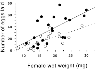
In the firefly species Photinus ignitus, the male transfers a large spermatophore to the female during mating. Rooney and Lewis (2002) wanted to know whether the extra resources from this "nuptial gift" enable the female to produce more offspring. They collected 40 virgin females and mated 20 of them to one male and 20 to three males. They then counted the number of eggs each female laid. Because fecundity varies with the size of the female, they analyzed the data using ancova, with female weight (before mating) as the independent measurement variable and number of eggs laid as the dependent measurement variable. Because the number of males has only two values ("one" or "three"), it is a nominal variable, not measurement.

The slopes of the two regression lines (one for single-mated females and one for triple-mated females) are not significantly different (F_{1, 36}=1.1, P=0.30). The Y intercepts are significantly different (F_{1, 36}=8.8, P=0.005); females that have mated three times have significantly more offspring than females mated once.

---

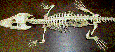
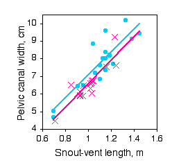
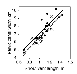
Paleontologists would like to be able to determine the sex of dinosaurs from their fossilized bones. To see whether this is feasible, Prieto-Marquez et al. (2007) measured several characters that are thought to distinguish the sexes in alligators (Alligator mississipiensis), which are among the closest living non-bird relatives of dinosaurs. One of the characters was pelvic canal width, which they wanted to standardize using snout-vent length.

The slopes of the regression lines are not significantly different (P=0.9101). The Y intercepts are significantly different (P=0.0267), indicating that male alligators of a given length have a significantly greater pelvic canal width. However, inspection of the graph shows that there is a lot of overlap between the sexes even after standardizing for sex, so it would not be possible to reliably determine the sex of a single individual with this character alone.

Graphing the results

You graph an ancova with a scattergraph, with the independent variable on the X axis and the dependent variable on the Y axis. Use a different symbol for each value of the nominal variable, as in the firefly graph above, where filled circles are used for the thrice-mated females and open circles are used for the once-mated females. To get this kind of graph in a spreadsheet, you would put all of the X values in column A, one set of Y values in column B, the next set of Y values in column C, and so on.

Most people plot the individual regression lines for each set of points, as shown in the firefly graph, even if the slopes are not significantly different. This lets people see how similar or different the slopes look. This is easy to do in a spreadsheet; just click on one of the symbols and choose "Add Trendline" from the Chart menu.

Similar tests

Another way to standardize one measurement variable by another is to take the ratio of the two. For example, let's say some neighborhood ruffians have been giving you the finger, and this inspires you to compare the middle-finger length of boys vs. girls. Obviously, taller children will tend to have longer middle fingers, so you want to standardize for height; you want to know whether boys and girls of the same height have different middle-finger lengths. A simple way to do this would be to divide the middle-finger length by the child's height and compare these ratios between boys and girls using a two-sample t–test.

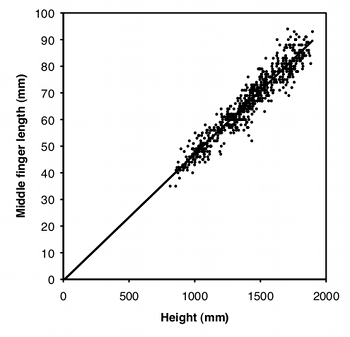
Using a ratio like this makes the statistics simpler and easier to understand, but you should only use ratios when the two measurement variables are isometric. This means that the ratio of Y over X does not change as X increases; in other words, the Y intercept of the regression line is 0. As you can see from the graph, middle-finger length in a sample of 645 boys (Snyder et al. 1977) does look isometric, so you could analyze the ratios. The average ratio in the Snyder et al. (1977) data set is 0.0472 for boys and 0.0470 for girls, and the difference is not significant (two-sample t–test, P=0.50).

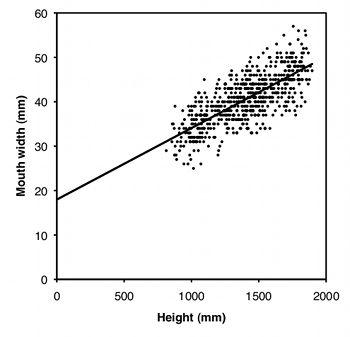
However, many measurements are allometric: the ratio changes as the X variable gets bigger. For example, let's say that in addition to giving you the finger, the rapscallions have been cursing at you, so you decide to compare the mouth width of boys and girls. As you can see from the graph, mouth width is very allometric; smaller children have bigger mouths as a proportion of their height. As a result, any difference between boys and girls in mouth width/height ratio could just be due to a difference in height between boys and girls. For data where the regression lines do not have a Y intercept of zero, you need to compare groups using ancova.

Sometimes the two measurement variables are just the same variable measured at different times or places. For example, if you measured the weights of two groups of individuals, put some on a new weight-loss diet and the others on a control diet, then weighed them again a year later, you could treat the difference between final and initial weights as a single variable, and compare the mean weight loss for the control group to the mean weight loss of the diet group using a one-way anova. The alternative would be to treat final and initial weights as two different variables and analyze using an ancova: you would compare the regression line of final weight vs. initial weight for the control group to the regression line for the diet group. The one-way anova would be simpler, and probably perfectly adequate; the ancova might be better, particularly if you had a wide range of initial weights, because it would allow you to see whether the change in weight depended on the initial weight.

How to do the test

Spreadsheet and web pages

Richard Lowry has made web pages that allow you to perform ancova with two, three or four groups, and a downloadable spreadsheet for ancova with more than four groups. You may cut and paste data from a spreadsheet to the web pages. In the results, the P value for "adjusted means" is the P value for the difference in the intercepts among the regression lines; the P value for "between regressions" is the P value for the difference in slopes.

R

Salvatore Mangiafico's R Companion has a sample R program for analysis of covariance.

SAS

Here's how to do analysis of covariance in SAS, using the cricket data from Walker (1962); I estimated the values by digitizing the graph, so the results may be slightly different from in the paper.

DATA crickets;   
   INPUT species $ temp pulse @@;   
DATALINES;
ex 20.8 67.9 ex 20.8  65.1 ex 24   77.3 ex 24    78.7 ex 24   79.4 
ex 24   80.4 ex 26.2  85.8 ex 26.2 86.6 ex 26.2  87.5 ex 26.2 89.1 
ex 28.4 98.6 ex 29   100.8 ex 30.4 99.3 ex 30.4 101.7 
niv 17.2  44.3 niv 18.3  47.2 niv 18.3  47.6 niv 18.3  49.6 
niv 18.9  50.3 niv 18.9  51.8 niv 20.4  60   niv 21    58.5 
niv 21    58.9 niv 22.1  60.7 niv 23.5  69.8 niv 24.2  70.9 
niv 25.9  76.2 niv 26.5  76.1 niv 26.5  77   niv 26.5  77.7 
niv 28.6  84.7
;
PROC GLM DATA=crickets;   
   CLASS species;   
   MODEL pulse=temp species temp*species;
PROC GLM DATA=crickets;   
   CLASS species;
   MODEL pulse=temp species;   
RUN;

The CLASS statement gives the nominal variable, and the MODEL statement has the Y variable to the left of the equals sign. The first time you run PROC GLM, the MODEL statement includes the X variable, the nominal variable, and the interaction term ("temp*species" in the example). This tests whether the slopes of the regression lines are significantly different. You'll see both Type I and Type III sums of squares; the Type III sums of squares are the correct ones to use:

Source         DF     Type III SS     Mean Square    F Value   Pr > F

temp           1     4126.440681     4126.440681    1309.61    <.0001
species        1        2.420117        2.420117       0.77    0.3885
temp*species   1        4.275779        4.275779       1.36    0.2542 slope P value

If the P value of the slopes is significant, you'd be done. In this case it isn't, so you look at the output from the second run of PROC GLM. This time, the MODEL statement doesn't include the interaction term, so the model assumes that the slopes of the regression lines are equal. This P value tells you whether the Y intercepts are significantly different:

Source         DF     Type III SS     Mean Square    F Value    Pr > F

temp           1     4376.082568     4376.082568    1371.35    <.0001
species        1      598.003953      598.003953     187.40    <.0001intercept P value

If you want the common slope and the adjusted means, add SOLUTION to the MODEL statement and another line with LSMEANS and the CLASS variable:

PROC GLM DATA=crickets;
   CLASS species;
   MODEL pulse=temp species/SOLUTION;
   LSMEANS species;

yields this as part of the output:

                                        Standard
Parameter             Estimate             Error    t Value    Pr > |t|

Intercept         -17.27619743 B      2.19552853      -7.87      <.0001
temp                3.60275287        0.09728809      37.03      <.0001
species   ex       10.06529123 B      0.73526224      13.69      <.0001
species   niv       0.00000000 B       .                .         .    

NOTE: The X'X matrix has been found to be singular, and a generalized 
inverse was used to solve the normal equations.  Terms whose 
estimates are followed by the letter 'B' are not uniquely estimable.

                     The GLM Procedure
                    Least Squares Means

                  species    pulse LSMEAN

                  ex           78.4067726
                  niv          68.3414814

Under "Estimate," 3.60 is the common slope. -17.27 is the Y intercept for the regression line for O. niveus. 10.06 means that the Y intercept for O. exclamationis is 10.06 higher (-17.27+10.06). Ignore the scary message about the matrix being singular.

If you have more than two regression lines, you can do a Tukey-Kramer test comparing all pairs of y-intercepts. If there were three cricket species in the example, you'd say "LSMEANS species/PDIFF ADJUST=TUKEY;".

Power analysis

You can't do a power analysis for ancova with G*Power, so I've prepared a spreadsheet to do power analysis for ancova, using the method of Borm et al. (2007). It only works for ancova with two groups, and it assumes each group has the same standard deviation and the same r². To use it, you'll need:

• the effect size, or the difference in Y intercepts you hope to detect;
• the standard deviation. This is the standard deviation of all the Y values within each group (without controlling for the X variable). For example, in the alligator data above, this would be the standard deviation of pelvic width among males, or the standard deviation of pelvic width among females.
• alpha, or the significance level (usually 0.05);
• power, the probability of rejecting the null hypothesis when the given effect size is the true difference (0.80 or 0.90 are common values);
• the r² within groups. For the alligator data, this would be the r² of pelvic width vs. snout-vent length among males, or the r² among females.

As an example, let's say you want to do a study with an ancova on pelvic width vs. snout-vent length in male and female crocodiles, and since you don't have any preliminary data on crocodiles, you're going to base your sample size calculation on the alligator data. You want to detect a difference in Y intercepts of 0.2 cm. The standard deviation of pelvic width in the male alligators is 1.45 and for females is 1.02; taking the average, enter 1.23 for standard deviation. The r² in males is 0.774 and for females it's 0.780, so enter the average (0.777) for r² in the form. With 0.05 for the alpha and 0.80 for the power, the result is that you'll need 133 male crocodiles and 133 female crocodiles.

References

Frog calls from Knapp, W.S. 2007. The Frogs and Toads of Georgia.

Alligator skeleton from University of Washington: Biology 453, Comparative Vertebrate Anatomy.

Borm, G.F., J. Fransen, and W.A.J.G. Lemmens. 2007. A simple sample size formula for analysis of covariance in randomized clinical trials. Journal of Clinical Epidemiology 60: 1234-1238.

Prieto-Marquez, A., P.M. Gignac, and S. Joshi. 2007. Neontological evaluation of pelvic skeletal attributes purported to reflect sex in extinct non-avian archosaurs. Journal of Vertebrate Paleontology 27: 603-609.

Rooney, J., and S.M. Lewis. 2002. Fitness advantage from nuptial gifts in female fireflies. Ecolological Entomology 27: 373-377.

Snyder, R. G., Schneider, L. W., Owings, C. L., Reynolds, H. M., Golomb, D. H., and Schork, M. A. 1977. Anthropometry of infants, children, and youths to age 18 for product safety designs. Warrendale, PA: Society for Automotive Engineers. [Snyder et al. data downloaded from Matthew Reed's Downloads Page]

Walker T. J. 1962. The taxonomy and calling songs of United States tree crickets (Orthoptera: Gryllidae: Oecanthinae). I. The genus Neoxabea and the niveus and varicornis groups of the genus Oecanthus. Annals of the Entomological Society of America 55: 303-322.

---

⇐ Previous topic|Next topic ⇒
Table of Contents

---

This page was last revised July 20, 2015. Its address is http://www.biostathandbook.com/ancova.html. It may be cited as:
McDonald, J.H. 2014. Handbook of Biological Statistics (3rd ed.). Sparky House Publishing, Baltimore, Maryland. This web page contains the content of pages 220-228 in the printed version.

©2014 by John H. McDonald. You can probably do what you want with this content; see the permissions page for details.