⇐ Previous topic|Next topic ⇒
Table of Contents
Homoscedasticity and heteroscedasticity
Summary
Parametric tests assume that data are homoscedastic (have the same standard deviation in different groups). Here I explain how to check this and what to do if the data are heteroscedastic (have different standard deviations in different groups).
Introduction
One of the assumptions of an anova and other parametric tests is that the within-group standard deviations of the groups are all the same (exhibit homoscedasticity). If the standard deviations are different from each other (exhibit heteroscedasticity), the probability of obtaining a false positive result even though the null hypothesis is true may be greater than the desired alpha level.
To illustrate this problem, I did simulations of samples from three populations, all with the same population mean. I simulated taking samples of 10 observations from population A, 7 from population B, and 3 from population C, and repeated this process thousands of times. When the three populations were homoscedastic (had the same standard deviation), the one-way anova on the simulated data sets were significant (P<0.05) about 5% of the time, as they should be. However, when I made the standard deviations different (1.0 for population A, 2.0 for population B, and 3.0 for population C), I got a P value less than 0.05 in about 18% of the simulations. In other words, even though the population means were really all the same, my chance of getting a false positive result was 18%, not the desired 5%.
There have been a number of simulation studies that have tried to determine when heteroscedasticity is a big enough problem that other tests should be used. Heteroscedasticity is much less of a problem when you have a balanced design (equal sample sizes in each group). Early results suggested that heteroscedasticity was not a problem at all with a balanced design (Glass et al. 1972), but later results found that large amounts of heteroscedasticity can inflate the false positive rate, even when the sample sizes are equal (Harwell et al. 1992). The problem of heteroscedasticity is much worse when the sample sizes are unequal (an unbalanced design) and the smaller samples are from populations with larger standard deviations; but when the smaller samples are from populations with smaller standard deviations, the false positive rate can actually be much less than 0.05, meaning the power of the test is reduced (Glass et al. 1972).
What to do about heteroscedasticity
You should always compare the standard deviations of different groups of measurements, to see if they are very different from each other. However, despite all of the simulation studies that have been done, there does not seem to be a consensus about when heteroscedasticity is a big enough problem that you should not use a test that assumes homoscedasticity.
If you see a big difference in standard deviations between groups, the first things you should try are data transformations. A common pattern is that groups with larger means also have larger standard deviations, and a log or square-root transformation will often fix this problem. It's best if you can choose a transformation based on a pilot study, before you do your main experiment; you don't want cynical people to think that you chose a transformation because it gave you a significant result.
If the standard deviations of your groups are very heterogeneous no matter what transformation you apply, there are a large number of alternative tests to choose from (Lix et al. 1996). The most commonly used alternative to one-way anova is Welch's anova, sometimes called Welch's t–test when there are two groups.
Non-parametric tests, such as the Kruskal–Wallis test instead of a one-way anova, do not assume normality, but they do assume that the shapes of the distributions in different groups are the same. This means that non-parametric tests are not a good solution to the problem of heteroscedasticity.
All of the discussion above has been about one-way anovas. Homoscedasticity is also an assumption of other anovas, such as nested and two-way anovas, and regression and correlation. Much less work has been done on the effects of heteroscedasticity on these tests; all I can recommend is that you inspect the data for heteroscedasticity and hope that you don't find it, or that a transformation will fix it.
Bartlett's test
There are several statistical tests for homoscedasticity, and the most popular is Bartlett's test. Use this test when you have one measurement variable, one nominal variable, and you want to test the null hypothesis that the standard deviations of the measurement variable are the same for the different groups.
Bartlett's test is not a particularly good one, because it is sensitive to departures from normality as well as heteroscedasticity; you shouldn't panic just because you have a significant Bartlett's test. It may be more helpful to use Bartlett's test to see what effect different transformations have on the heteroscedasticity; you can choose the transformation with the highest (least significant) P value for Bartlett's test.
An alternative to Bartlett's test that I won't cover here is Levene's test. It is less sensitive to departures from normality, but if the data are approximately normal, it is less powerful than Bartlett's test.
While Bartlett's test is usually used when examining data to see if it's appropriate for a parametric test, there are times when testing the equality of standard deviations is the primary goal of an experiment. For example, let's say you want to know whether variation in stride length among runners is related to their level of experience—maybe as people run more, those who started with unusually long or short strides gradually converge on some ideal stride length. You could measure the stride length of non-runners, beginning runners, experienced amateur runners, and professional runners, with several individuals in each group, then use Bartlett's test to see whether there was significant heterogeneity in the standard deviations.
How to do Bartlett's test
Spreadsheet
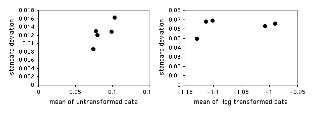
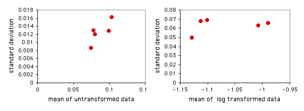
I have put together a spreadsheet that performs Bartlett's test for homogeneity of standard deviations for up to 1000 observations in each of up to 50 groups. It allows you to see what the log or square-root transformation will do. It also shows a graph of the standard deviations plotted vs. the means. This gives you a quick visual display of the difference in amount of variation among the groups, and it also shows whether the mean and standard deviation are correlated.
Entering the mussel shell data from the one-way anova web page into the spreadsheet, the P values are 0.655 for untransformed data, 0.856 for square-root transformed, and 0.929 for log-transformed data. None of these is close to significance, so there's no real need to worry. The graph of the untransformed data hints at a correlation between the mean and the standard deviation, so it might be a good idea to log-transform the data:

Web page
There is web page for Bartlett's test that will handle up to 14 groups. You have to enter the variances (not standard deviations) and sample sizes, not the raw data.
SAS
You can use the HOVTEST=BARTLETT option in the MEANS statement of PROC GLM to perform Bartlett's test. This modification of the program from the one-way anova page does Bartlett's test.
PROC GLM DATA=musselshells;
  CLASS location;
  MODEL aam = location;
  MEANS location / HOVTEST=BARTLETT;
run;
References
Glass, G.V., P.D. Peckham, and J.R. Sanders. 1972. Consequences of failure to meet assumptions underlying fixed effects analyses of variance and covariance. Review of Educational Research 42: 237-288.
Harwell, M.R., E.N. Rubinstein, W.S. Hayes, and C.C. Olds. 1992. Summarizing Monte Carlo results in methodological research: the one- and two-factor fixed effects ANOVA cases. Journal of Educational Statistics 17: 315-339.
Lix, L.M., J.C. Keselman, and H.J. Keselman. 1996. Consequences of assumption violations revisited: A quantitative review of alternatives to the one-way analysis of variance F test. Review of Educational Research 66: 579-619.
⇐ Previous topic|Next topic ⇒
Table of Contents
This page was last revised December 4, 2014. Its address is http://www.biostathandbook.com/homoscedasticity.html. It may be cited as:
McDonald, J.H. 2014. Handbook of Biological Statistics (3rd ed.). Sparky House Publishing, Baltimore, Maryland. This web page contains the content of pages 137-139 in the printed version.
©2014 by John H. McDonald. You can probably do what you want with this content; see the permissions page for details.

